

Anomalies detection problems arises in so many applications for example in finance, health, defense and internal security, consumer home safety, manufacturing and Industry.
Our focus is on detecting anomalies in credit card transactions. Credit card fraud is on the increase as technology develops. The cost to both business and consumer from this type of fraud costs billions of dollars every year.

Fraudsters are continually finding new ways to commit their illegal activities. As a result has become essential for financial Institutions of businesses to develop advanced fraud detection techniques to counter the threat of fraudulent credit card transactions and identify theft and keep losses to a minimum.
In credit card anomaly detection, we know what the true positive are. How? Customers tell us. So we can use a supervised learning approach because the true class is self revealing. Some of the main issues we would encounter are;
- Severe class imbalance; fraudulent transactions are rare.
- Severe class overlap; fraudulent transactions and normal transactions are similar.
- Concept drift; fraudsters may change their patterns of attack.
- Uncertainty around the model.
What is an anomaly?
An anomaly is a "deviation" from the norm. Many scientific and engineering fields are based on the assumption that "processes" or "behaviors" exist in nature that follow certain rules and principles resulting in a well defined system manifested in observable data. These describes the normal behavior of a system and any deviation from this, is abnormal, hence we say that the system exists in an abnormal state.The task of anomaly detection is to detect those deviations from the norm. This poses an interesting problem, "what definition permits us to evaluate how similar/dissimilar two data points are from one another."
When applying anomaly detection algorithms, there are three possible scenarios. The algorithm for some input X produces;
1. Correct Prediction: Detected abnormalities in the data correspond exactly to the abnormalities in the process.
2. False Positives: The process continues to be normal but unexpected data values are observed due to noise.
3. False Negatives: The process becomes abnormal but the consequences are not registered in the abnormal data due to the sign of abnormality being similar to the normal process.
Most real life systems are such that 100% correct prediction is impossible. A common approach is to produce probability of a process being abnormal, this provides a starting point for human intervention and analysis.
What is a norm?
We have used the word "Normal" without a clear and concise definition. The mean, median and mode have long been used to capture the "norm" associated with distributions and the distance(deviation) from the point to its measure of central tendency is used to assess the degree to which the point is "abnormal".
The use of distances functions such as Euclidean distance and Mahalanobis distance which we shall define shortly with standard deviation along each dimensions removes the potential confusion that would have resulted due to in-commensurable dimensions.
The mahalanobis distance function is a measure of the distance between a point P and a distribution D. It measures how many standard deviations P is away from the mean of D. This can also be defined as a dissimilarity measure between two random vectors x and y of the same distribution with the covariances S.
The euclidean distance between two points in euclidean space is the length of a line segment between the two points. It is similar to the famous Pythagorean theorem.
Anomaly detection approaches
Anomaly detection can be classified as
Distance Based: Points that are further from others are considered more anomalous.
Density Based: Point that are relatively low density regions are considered more anomalous.
Rank Based: The most anomalous points are those whose nearest neighbors others as nearest neighbors. For each of the approaches, the problem may be supervised, semi-supervised or unsupervised.
In Supervised, the labels are known for a set of "training" data and all evaluation are done with respect to the training data. In the unsupervised case, no such labels are known, so distances and comparisons are with respect to the entire data set. In semi-supervised, labels are known for some data but for not for most others.
Metrics for measurement
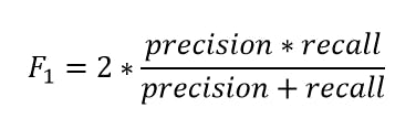
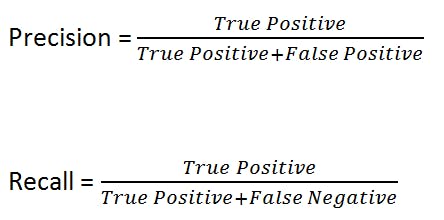
To evaluate the performance of the algorithm, three metrics are of relative importance: Precision, Recall, F1 score. The precision tells us how precise our model is in predicting the positive case while the recall measures how well a model "recalls" all positive case. An example can help illustrate this; A dataset contains 1, 000, 000 transactions of which 200 are fraudulent, an algorithm that considers all transactions as fraudulent has a precision of 0.0002 and a recall of 1.0.
When we increase precision, recall suffers. In some situations, recall is much important than precision. We might want our algorithm to flag down all fraudulent transactions but it could raise few false alarms. A simplification of precision and recall is f1 score which is just the harmonic mean of precision and recall.